Detect Cycle in Undirected Graph

Note: An undirected graph is basically the same as a directed graph with bidirectional connections (= two connections in opposite directions) between the connected nodes.

DFS

Here, if neighbour is not parent and still visited, that means its a cycle.

• Iterate over all the nodes of the graph and Keep a visited array visited[] to track the visited nodes.
• Run a Depth First Traversal on the given subgraph connected to the current node and pass the parent of the current node. In each recursive
  • Set visited[root] as 1.
  • Iterate over all adjacent nodes of the current node in the adjacency list
    • If it is not visited then run DFS on that node and return true if it returns true.
    • Else if the adjacent node is visited and not the parent of the current node then return true.
  • Return false.

def DFS(graph, v, discovered, parent):
    discovered[v] = True
    for w in graph.adjList[v]:
        if not discovered[w]:
            if DFS(graph, w, discovered, v):
                return True
        elif w != parent: 
            return True
    return False

discovered = [False] * N
DFS(graph, 1, discovered, -1)

Time Complexity: O(V + E), the Time Complexity of this method is the same as the time complexity of DFS traversal which is O(V+E).
Auxiliary Space: O(V). To store the visited O(V) space is needed.

BFS

For every visited vertex ‘v’, if there is an adjacent ‘u’ such that u is already visited and u is not a parent of v, then there is a cycle in the graph. If we don’t find such an adjacent for any vertex, we say that there is no cycle.
We use a parent array to keep track of the parent vertex for a vertex so that we do not consider the visited parent as a cycle.

def isCyclicConnected(adj: list, s, V, visited: list):
    parent = [-1] * V
    q = deque()
    visited[s] = True
    q.append(s)
    while q != []:
        u = q.pop()
        # Get all adjacent vertices of the dequeued vertex u. If a adjacent has not been visited,
        # then mark it visited and enqueue it. We also mark parent so that parent is not considered for cycle.
        for v in adj[u]:
            if not visited[v]:
                visited[v] = True
                q.append(v)
                parent[v] = u
            elif parent[u] != v:
                return True
 
    return False
 
def isCyclicDisconnected(adj: list, V):
    visited = [False] * V
    for i in range(V):
        if not visited[i] and isCyclicConnected(adj, i, V, visited):
            return True
    return False

Time Complexity: O(V + E), the Time Complexity of this method is the same as the time complexity of BFS traversal which is O(V+E).
Auxiliary Space: O(V). To store the visited O(V) space is needed + O(V) by queue.

Detect Cycle in Directed Graph

DFS

To find cycle in a directed graph we can use the Depth First Traversal (DFS) technique. It is based on the idea that there is a cycle in a graph only if there is a back edge [i.e., a node points to one of its ancestors] present in the graph.
To detect a back edge, we need to keep track of the nodes visited till now and the nodes that are in the current recursion stack [i.e., the current path that we are visiting]. If during recursion, we reach a node that is already in the recursion stack, there is a cycle present in the graph.
Follow the below steps to Implement the idea:

• Create a recursive dfs function that has the following parameters – current vertex, visited array, and recursion stack.
• Mark the current node as visited and also mark the index in the recursion stack.
• Iterate a loop for all the vertices and for each vertex, call the recursive function if it is not yet visited (This step is done to make sure that if there is a forest of graphs, we are checking each forest):
  • In each recursion call, Find all the adjacent vertices of the current vertex which are not visited:
    • If an adjacent vertex is already marked in the recursion stack then return true.
    • Otherwise, call the recursive function for that adjacent vertex.
  • While returning from the recursion call, unmark the current node from the recursion stack, to represent that the current node is no longer a part of the path being traced.
• If any of the functions returns true, stop the future function calls and return true as the answer.

    def isCyclicUtil(self, v, visited, recStack):
        visited[v] = True
        recStack[v] = True
 
        for neighbour in self.graph[v]:
            if visited[neighbour] == False:
                if self.isCyclicUtil(neighbour, visited, recStack) == True:
                    return True
            elif recStack[neighbour] == True:
                return True
 
        # The node needs to be popped from recursion stack before function ends
        recStack[v] = False
        return False
 
    def isCyclic(self):
        visited = [False] * (self.V + 1)
        recStack = [False] * (self.V + 1)
        for node in range(self.V):
            if visited[node] == False:
                if self.isCyclicUtil(node, visited, recStack) == True:
                    return True
        return False

Time Complexity: O(V + E), the Time Complexity of this method is the same as the time complexity of DFS traversal which is O(V+E).
Auxiliary Space: O(V). To store the visited and recursion stack O(V) space is needed.

BFS by (Topological sorting) or (KAHN's Algo)

Here we are using Kahn’s algorithm for topological sorting, if it successfully removes all vertices from the graph, it’s a DAG with no cycles. If there are remaining vertices with in-degrees greater than 0, it indicates the presence of at least one cycle in the graph. Hence, if we are not able to get all the vertices in topological sorting then there must be at least one cycle.
To understand Topological sorting, it's the next topic.

def isCyclic(self):
        inDegree = [0] * self.V
        q = deque()
        visited = 0
 
        # Calculate in-degree of each vertex
        for u in range(self.V):
            for v in self.adj[u]:
                inDegree[v] += 1
 
        # Enqueue vertices with 0 in-degree
        for u in range(self.V):
            if inDegree[u] == 0:
                q.append(u)
 
        # BFS traversal
        while q:
            u = q.popleft()
            visited += 1
 
            # Reduce in-degree of adjacent vertices
            for v in self.adj[u]:
                inDegree[v] -= 1
                # If in-degree becomes 0, enqueue the vertex
                if inDegree[v] == 0:
                    q.append(v)
		 # if not all vertex were popped, that means vertex with zero degrees are still left.
        return visited != self.V  

Time Complexity: O(V + E), the Time Complexity of this method is the same as the time complexity of BFS traversal which is O(V+E).
Auxiliary Space: O(V). To store the visited O(V) space is needed + O(V) by queue.

Topological sorting

Topological sorting for Directed Acyclic Graph (DAG) is a linear ordering of vertices such that for every directed edge u-v, vertex u comes before v in the ordering.

Note: Topological Sorting for a graph is not possible if the graph is not a DAG.

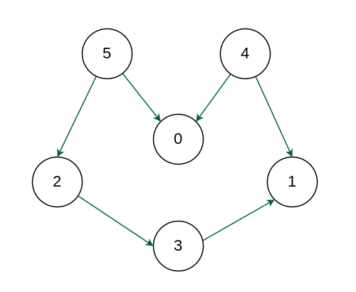
Output: 5 4 2 3 1 0
Explanation: The first vertex in topological sorting is always a vertex with an in-degree of 0 (a vertex with no incoming edges). A topological sorting of the following graph is “5 4 2 3 1 0”. There can be more than one topological sorting for a graph. Another topological sorting of the following graph is “4 5 2 3 1 0”.

DFS

In topological sorting:

• We use a temporary stack.
• We don’t print the vertex immediately,
• We first recursively call topological sorting for all its adjacent vertices, then push it to a stack.
• Finally, print the contents of the stack.
  Note: A vertex is pushed to stack only when all of its adjacent vertices (and their adjacent vertices and so on) are already in the stack

Approach:

• Create a stack to store the nodes.
• Initialize visited array of size N to keep the record of visited nodes.
• Run a loop from 0 till N :
• if the node is not marked True in visited array then call the recursive function for topological sort and perform the following steps:
  • Mark the current node as True in the visited array.
  • Run a loop on all the nodes which has a directed edge to the current node
  • if the node is not marked True in the visited array:
    • Recursively call the topological sort function on the node
  • Push the current node in the stack.
• Print all the elements in the stack.

Illustration: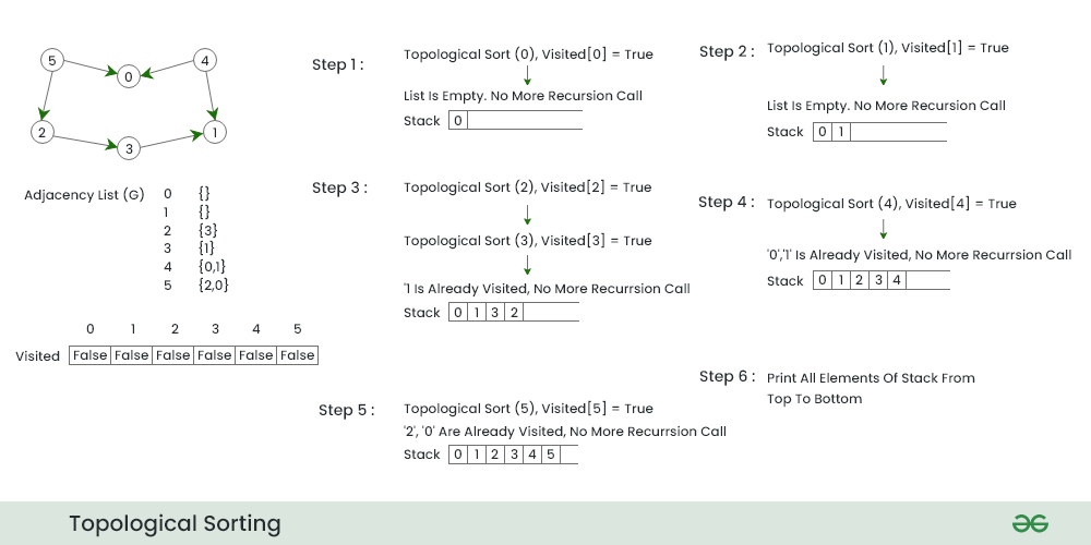

def topologicalSortUtil(self, v, visited, stack):
        visited[v] = True
        for i in self.graph[v]:
            if visited[i] == False:
                self.topologicalSortUtil(i, visited, stack)
 
        # Push current vertex to stack which stores result
        stack.append(v)

    def topologicalSort(self):
        visited = [False]*self.V
        stack = []
 
        for i in range(self.V):
            if visited[i] == False:
                self.topologicalSortUtil(i, visited, stack)
        print(stack[::-1])  # return list in reverse order

BFS (KAHN's ALGO)

A DAG G has at least one vertex with in-degree 0 and one vertex with out-degree 0.
Proof: There’s a simple proof to the above fact that a DAG does not contain a cycle which means that all paths will be of finite length. Now let S be the longest path from u(source) to v(destination). Since S is the longest path there can be no incoming edge to u and no outgoing edge from v, if this situation had occurred then S would not have been the longest path
=> indegree(u) = 0 and outdegree(v) = 0
Topological sorting is a kind of dependencies problem so, we can start with the tasks which do not have any dependencies and can be done straight away or simply if we talk about in the term of node,

• We will always try to execute those nodes that have outdegree 0.
• Then after execution of all those 0 outdegrees, we will execute which are directly dependent on currently resolved tasks (currently resolved tasks’ outdegrees will become 0 now) and so on will execute all other tasks.

Algorithm: Steps involved in finding the topological ordering of a DAG:
Step-1: Compute in-degree (number of incoming edges) for each of the vertex present in the DAG and initialize the count of visited nodes as 0.
Step-2: Pick all the vertices with in-degree as 0 and add them into a queue (Enqueue operation)
Step-3: Remove a vertex from the queue (Dequeue operation) and then.
* Increment the count of visited nodes by 1.
* Decrease in-degree by 1 for all its neighbouring nodes.
* If the in-degree of neighbouring nodes is reduced to zero, then add it to the queue.
Step 4: Repeat Step 3 until the queue is empty.
Step 5: If the count of visited nodes is not equal to the number of nodes in the graph then the topological sort is not possible for the given graph.

def topologicalSort(self):

        in_degree = [0]*(self.V)
        for i in self.graph:
            for j in self.graph[i]:
                in_degree[j] += 1
 
        # Create an queue and enqueue all vertices witt indegree 0
        queue = []
        for i in range(self.V):
            if in_degree[i] == 0:
                queue.append(i)
 
        # Initialize count of visited vertices
        cnt = 0
		
        top_order = []
        while queue:
            u = queue.pop(0)
            top_order.append(u)
            for i in self.graph[u]:
                in_degree[i] -= 1
                if in_degree[i] == 0:
                    queue.append(i)
 
            cnt += 1
 
        # Check if there was a cycle
        if cnt != self.V:
            print ("There exists a cycle in the graph")
        else :
            print (top_order)

Time Complexity: O(V+E). The outer for loop will be executed V number of times and the inner for loop will be executed E number of times.
Auxiliary Space: O(V). The queue needs to store all the vertices of the graph. So the space required is O(V)

Bipartite Graph

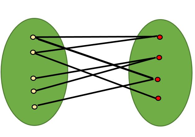
A Bipartite Graph is a graph whose vertices can be divided into two independent sets, U and V such that every edge (u, v) either connects a vertex from U to V or a vertex from V to U. In other words, for every edge (u, v), either u belongs to U and v to V, or u belongs to V and v to U. We can also say that there is no edge that connects vertices of same set.

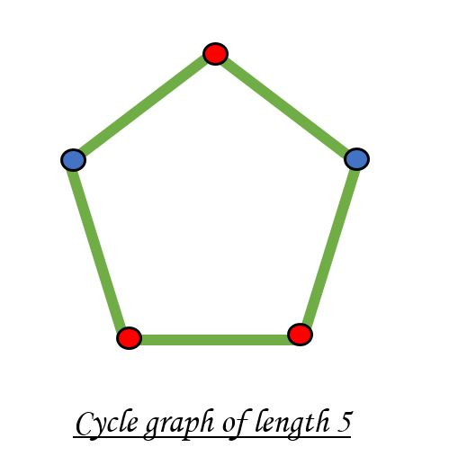
A bipartite graph is possible if the graph coloring is possible using two colors such that vertices in a set are colored with the same color. Note that it is possible to color a cycle graph with even cycle using two colors. For example, see the following graph.

It is not possible to color a cycle graph with odd cycle using two colors.

Following is a simple algorithm to find out whether a given graph is Bipartite or not using Breadth First Search (BFS).

1. Assign RED color to the source vertex (putting into set U).
2. Color all the neighbors with BLUE color (putting into set V).
3. Color all neighbor’s neighbor with RED color (putting into set U).
4. This way, assign color to all vertices such that it satisfies all the constraints of m way coloring problem where m = 2.
5. While assigning colors, if we find a neighbor which is colored with same color as current vertex, then the graph cannot be colored with 2 vertices (or graph is not Bipartite)

    def isBipartiteUtil(self, src):
        queue = []
        queue.append(src)
        while queue:
            u = queue.pop()
 
            # Return false if there is a self-loop
            if self.graph[u][u] == 1:
                return False
 
            for v in range(self.V):
                if (self.graph[u][v] == 1 and
                        self.colorArr[v] == -1):
                    self.colorArr[v] = 1 - self.colorArr[u]
                    queue.append(v)
                elif (self.graph[u][v] == 1 and
                      self.colorArr[v] == self.colorArr[u]):
                    return False
        return True
 
    def isBipartite(self):
        self.colorArr = [-1 for i in range(self.V)]
        for i in range(self.V):
            if self.colorArr[i] == -1:
                if not self.isBipartiteUtil(i):
                    return False
        return True

Time complexity: O(E+V).
Auxiliary Space: O(V), because we have a V-size array.

Can DFS algorithm be used to check the bipartite-ness of a graph? If yes, how?
Explanation:
The algorithm can be described as follows:
Step 1: To perform a DFS traversal, we require a starting node and an array to track visited nodes.
However, instead of using a visited array, we will utilize a color array where each node is initially assigned the value -1 to indicate that it has not been colored yet.
Step 2: In the DFS function call, it is important to pass the assigned color value and store it in the color array.
We will attempt to color the nodes using 0 and 1, although alternative colors can also be chosen.
Step 3: During the DFS traversal, For each uncolored node encountered, we assign it the opposite color of its current node.
Step 4: If, at any point, we encounter an adjacent node in the adjacency list that has already been colored and shares
the same color as the current node, it implies that coloring is not possible.
Consequently, we return false, indicating that the given graph is not bipartite. Otherwise, we continue returning true.

def colorGraph(G, color, pos, c): 
    if color[pos] != -1 and color[pos] != c: 
        return False
    # color this pos as c and all its neighbours and 1-c 
    color[pos] = c 
    ans = True
    for i in range(0, V): 
        if G[pos][i]: 
            if color[i] == -1: 
                ans &= colorGraph(G, color, i, 1-c) 
            if color[i] !=-1 and color[i] != 1-c: 
                return False
        if not ans: 
            return False
    return True
  
def isBipartite(G): 
    color = [-1] * V
    pos = 0
    # two colors 1 and 0 
    return colorGraph(G, color, pos, 1)

Shortest Path Alogrithms

1. Dijkstra’s Algorithm

Limitations:

• Single Source Shortest Path(from a single source, tell shortest path to every node)
• Only (non negative edge weights) -> (0, +ve)
• Can work for both Directed/Undirected graphs.

Initial configuration:
Source Node: Before starting off with the Algorithm, we need to define a source node from which the shortest distances to every other node would be calculated.
Priority Queue: Define a Priority Queue which would contain pairs of the type {dist, node}, where ‘dist’ indicates the currently updated value of the shortest distance from the source to the ‘node’.
Dist Array: Define a dist array initialized with a large integer number at the start indicating that the nodes are unvisited initially. This array stores the shortest distances to all the nodes from the source node.
The Algorithm consists of the following steps :

• We would be using a min-heap and a distance array of size V (where ‘V’ are the number of nodes in the graph) initialized with infinity (indicating that at present none of the nodes are reachable from the source node) and initialize the distance to source node as 0.
• We push the source node to the queue along with its distance which is also 0.
• For every node at the top of the queue, we pop the element out and look out for its adjacent nodes. If the current reachable distance is better than the previous distance indicated by the distance array, we update the distance and push it into the queue.

A node with a lower distance would be at the top of the priority queue as opposed to a node with a higher distance because we are using a min-heap. By following step 3, until our queue becomes empty, we would get the minimum distance from the source node to all other nodes. We can then return the distance array.

import heapq

class Solution:
    def dijkstra(self, V, adj, S):
        pq = []
        distTo = [float('inf')] * V
        parent = [-1] * V  # To store the path
        distTo[S] = 0
        heapq.heappush(pq, (0, S))

        while pq:
            dis, node = heapq.heappop(pq)

            for neighbor in adj[node]:
                v = neighbor[0]
                w = neighbor[1]

                if dis + w < distTo[v]:
                    distTo[v] = dis + w
                    parent[v] = node
                    heapq.heappush(pq, (dis + w, v))

        return distTo, parent

    def print_path(self, parent, node):
        path = []
        while node != -1:
            path.append(node)
            node = parent[node]
        path.reverse()
        return path


# Driver code
if __name__ == "__main__":
    V, E, S = 3, 3, 2
    adj = [[] for _ in range(V)]

    # Edges (directed or undirected depending on context)
    adj[0].append([1, 1])
    adj[0].append([2, 6])
    adj[1].append([2, 3])
    adj[1].append([0, 1])
    adj[2].append([1, 3])
    adj[2].append([0, 6])

    obj = Solution()
    dist, parent = obj.dijkstra(V, adj, S)

    print("Shortest distances from source:", S)
    for i in range(V):
        print(f"Node {i}: Distance = {dist[i]}, Path = {obj.print_path(parent, i)}")

Time Complexity: O( E log(V) ), Where E = Number of edges and V = Number of Nodes.

Space Complexity: O( |E| + |V| ), Where E = Number of edges and V = Number of Nodes.

2. Bellman Ford Algorithm

Limitations:

• Single Source Shortest Path(from a single source, tell shortest path to every node)
• Works on all type of edge weights (-ve, 0, +ve)
• Can work for both only Directed graphs.
• Can give wrong answers with negative weighted cycles.
• Helps a lot in detecting Negative Cycles in graph.

The bellman-Ford algorithm helps to find the shortest distance from the source node to all other nodes. But, we have already learned Dijkstra’s algorithm (Dijkstra’s algorithm article link) to fulfill the same purpose. Now, the question is how this algorithm is different from Dijkstra’s algorithm.

While learning Dijkstra’s algorithm, we came across the following two situations, where Dijkstra’s algorithm failed:

If the graph contains negative edges.
If the graph has a negative cycle (In this case Dijkstra’s algorithm fails to minimize the distance, keeps on running, and goes into an infinite loop. As a result it gives TLE error).

Negative Cycle: A cycle is called a negative cycle if the sum of all its weights becomes negative. The following illustration is an example of a negative cycle:

Bellman-Ford’s algorithm successfully solves these problems. It works fine with negative edges as well as it is able to detect if the graph contains a negative cycle. But this algorithm is only applicable for directed graphs.
In order to apply this algorithm to an undirected graph, we just need to convert the undirected edges into directed edges like the following:

After doing this we can apply Bellman ford on undirected graphs too.

Intuition:
In this algorithm, the edges can be given in any order. The intuition is to relax all the edges for N-1( N = no. of nodes) times sequentially. After N-1 iterations, we should have minimized the distance to every node.

Let’s understand what the relaxation of edges means using an example.

Let’s consider the above graph with dist[u], dist[v], and wt. Here, wt is the weight of the edge and dist[u] signifies the shortest distance to reach node u found until now. Similarly, dist[v](maybe infinite) signifies the shortest distance to reach node v found until now. If the distance to reach v through u(i.e. dist[u] + wt) is smaller than dist[v], we will update the value of dist[v] with (dist[u] + wt). This process of updating the distance is called the relaxation of edges.

We will apply the above process(i.e. minimizing the distance to reach every node) N-1 times in the Bellman-Ford algorithm.

Two follow-up questions about the algorithm:
1. Why do we need exact N-1 iterations?
Let’s try to first understand this using an example:

• In the above graph, the algorithm will minimize the distance of the ith node in the ith iteration like dist[1] will be updated in the 1st iteration, dist[2] will be updated in the 2nd iteration, and so on. So we will need a total of 4 iterations(i.e. N-1 iterations) to minimize all the distances as dist[0] is already set to 0.
  Note: Points to remember since, in a graph of N nodes we will take at most N-1 edges to reach from the first to the last node, we need exact N-1 iterations. It is impossible to draw a graph that takes more than N-1 edges to reach any node.

2. How to detect a negative cycle in the graph?

• We know if we keep on rotating inside a negative cycle, the path weight will be decreased in every iteration. But according to our intuition, we should have minimized all the distances within N-1 iterations(that means, after N-1 iterations no relaxation of edges is possible).
• In order to check the existence of a negative cycle, we will relax the edges one more time after the completion of N-1 iterations. And if in that Nth iteration, it is found that further relaxation of any edge is possible, we can conclude that the graph has a negative cycle. Thus, the Bellman-Ford algorithm detects negative cycles.

Approach:
Initial Configuration:
distance array(dist[ ]): The dist[] array will be initialized with infinity, except for the source node as dist[src] will be initialized to 0.

The algorithm steps will be the following:

• First, we will initialize the source node in the distance array to 0 and the rest of the nodes to infinity.
• Then we will run a loop for N-1 times.
• Inside that loop, we will try to relax every given edge.
  For example, one of the given edge information is like (u, v, wt), where u = starting node of the edge, v = ending node, and wt = edge weight. For all edges like this we will be checking if node u is reachable and if the distance to reach v through u is less than the distance to v found until now(i.e. dist[u] and dist[u]+ wt < dist[v]).
• After repeating the 3rd step for N-1 times, we will apply the same step one more time to check if the negative cycle exists. If we found further relaxation is possible, we will conclude the graph has a negative cycle and from this step, we will return a distance array of -1(i.e. minimization of distances is not possible).
• Otherwise, we will return the distance array which contains all the minimized distances.

def BellmanFord(self, src):
        dist = [float("Inf")] * self.V
        dist[src] = 0
 
        # Relax all edges |V| - 1 times. A simple shortest path from src to any 
		# other vertex can have at-most |V| - 1 edges
        for _ in range(self.V - 1):
            # Update dist value and parent index of the adjacent vertices of
            # the picked vertex. Consider only those vertices which are still in queue
            for u, v, w in self.graph:
                if dist[u] != float("Inf") and dist[u] + w < dist[v]:
                    dist[v] = dist[u] + w
 
        # check for negative-weight cycles. The above step guarantees
        # shortest distances if graph doesn't contain negative weight cycle.
        # If we get a shorter path, then there is a cycle.
        for u, v, w in self.graph:
            if dist[u] != float("Inf") and dist[u] + w < dist[v]:
                print("Graph contains negative weight cycle")
                return
 
        # print all distance
        self.printArr(dist)

Time Complexity when graph is connected:
Best Case: O(E), when distance array after 1st and 2nd relaxation are same , we can simply stop further processing
Average Case: O(VE)
Worst Case: O(VE)
Time Complexity when graph is disconnected:
All the cases: O(E*(V^2))
Auxiliary Space: O(V), where V is the number of vertices in the graph.

3. Floyd Warshall Algorithm

Limitations:

• Multi Source Shortest Path(shortest distances between every pair of vertices )
• Works on all type of edge weights (-ve, 0, +ve)
• Can work for both only Directed graphs.
• Can give wrong answers with negative weighted cycles.
• Helps a lot in detecting Negative Cycles in graph.

Basically, the Floyd Warshall algorithm is a multi-source shortest path algorithm and it helps to detect negative cycles as well. The shortest path between node u and v necessarily means the path(from u to v) for which the sum of the edge weights is minimum.

In Floyd Warshall’s algorithm, we need to check every possible path going via each possible node. And after checking every possible path, we will figure out the shortest path(a kind of brute force approach to find the shortest path). Let’s understand it using the following illustration:

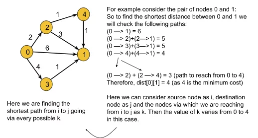
From the above example we can derive the following formula:
matrix[i][j] =min(matrix[i][j], matrix[i ][k]+matrix[k][j]), where i = source node, j = destination node, and k = the node via which we are reaching from i to j.

Here we will calculate dist[i][j] for every possible node k (k = 0, 1….V, where V = no. of nodes), and will select the minimum value as our result.

In order to apply this algorithm to an undirected graph, we just need to convert the undirected edges into directed edges.

Note:

• Until now, to store a graph we have used the adjacency list. But in this algorithm, we are going to use the adjacency matrix method.
• One additional point to remember is that the cost of reaching a node from itself must always be 0 i.e. dist[i][i] = 0, where i = current node.

Intuition:
The intuition is to check all possible paths between every possible pair of nodes and to choose the shortest one. Checking all possible paths means going via each and every possible node.

The follow-up questions for interviews:
1. How to detect a negative cycle using the Floyd Warshall algorithm?

We have previously said that the cost of reaching a node from itself must be 0. But in the above graph, if we try to reach node 0 from itself we can follow the path: 0->1->2->0. In this case, the cost to reach node 0 from itself becomes -3 which is less than 0. This is only possible if the graph contains a negative cycle.
So, if we find that the cost of reaching any node from itself is less than 0, we can conclude that the graph has a negative cycle.

2. What will happen if we will apply Dijkstra’s algorithm for this purpose?

• If the graph has a negative cycle: We cannot apply Dijkstra’s algorithm to the graph which contains a negative cycle. It will give TLE error in that case.
• If the graph does not contain a negative cycle: In this case, we will apply Dijkstra’s algorithm for every possible node to make it work like a multi-source shortest path algorithm like Floyd Warshall. The time complexity of Floyd Warshall is O(V3)(Which we will discuss later) whereas if we apply Dijkstra’s algorithm for the same purpose the time complexity reduces to O(V*(E*logV)) (where v = no. of vertices).

Approach:
The algorithm is not much intuitive as the other ones’. It is more of a brute force, where all combinations of paths have been tried to get the shortest paths. Nothing to panic much with the intuition, it is a simple brute force approach on all paths. Focus on the three ‘for’ loops.

Formula:
matrix[i][j] =min(matrix[i][j], matrix[i ][k]+matrix[k][j]), where i = source node,
j = destination node and k = the node via which we are reaching from i to j.

The algorithm steps are as follows:
Initial Configuration:
Adjacency Matrix: The adjacency matrix should store the edge weights for the given edges and the rest of the cells must be initialized with infinity().

1. After having set the adjacency matrix accordingly, we will run a loop from 0 to V-1(V = no. of vertices). In the kth iteration, this loop will help us to check the path via node k for every possible pair of nodes. Basically, this loop will change the value of k in the formula.
2. Inside the loop, there will be two nested loops for generating every possible pair of nodes(Nothing but to visit each cell of a 2D matrix using the nested loop). Among these two loops, the first loop will change the value of i and the second one will change the value of j in the formula.
3. Inside these nested loops, we will apply the above formula to calculate the shortest distance between the pair of nodes.
4. Finally, the adjacency matrix will store all the shortest paths. For example, matrix[i][j] will store the shortest path from node i to node j.

If we want to check for a negative cycle:
After completing the steps(outside those three loops), we will run a loop and check if any cell having the row and column the same(i = j) contains a value less than 0.

def floydWarshall(graph):
    """ dist[][] will be the output matrix that will finally have the shortest distances
	between every pair of vertices """
	""" initializing the solution matrix same as input graph matrix OR we can say that the initial 
    values of shortest distances are based on shortest paths considering no intermediate vertices """
 
    dist = list(map(lambda i: list(map(lambda j: j, i)), graph))
	for i in range(N):
		for j in range(N):
			if graph[i][j] == -1:
				dist[i][j] = 10**9
			if i==j: dist[i][j] = 0
 
    """ Add all vertices one by one  to the set of intermediate vertices.  
	 ---> Before start of an iteration, we have shortest distances between all pairs of vertices 
     such that the shortest distances consider only the vertices in the set 
    {0, 1, 2, .. k-1} as intermediate vertices.
      ----> After the end of a iteration, vertex no. k is added to the set of intermediate vertices and the 
    set becomes {0, 1, 2, .. k}
    """
    for k in range(V):
        # pick all vertices as source one by one
        for i in range(V):
            # Pick all vertices as destination for the
            # above picked source
            for j in range(V):
                # If vertex k is on the shortest path from
                # i to j, then update the value of dist[i][j]
                dist[i][j] = min(dist[i][j],
                                 dist[i][k] + dist[k][j]
                                 )
    printSolution(dist)

Time Complexity: O(V3), as we have three nested loops each running for V times, where V = no. of vertices.

Space Complexity: O(V2), where V = no. of vertices. This space complexity is due to storing the adjacency matrix of the given graph.

4. Shortest Path in DAG (Not an Algo, but a better TC approach for specific case.)

Intuition:
Finding the shortest path to a vertex is easy if you already know the shortest paths to all the vertices that can precede it. Processing the vertices in topological order ensures that by the time you get to a vertex, you’ve already processed all the vertices that can precede it which reduces the computation time significantly. In this approach, we traverse the nodes sequentially according to their reachability from the source.

Dijkstra’s algorithm is necessary for graphs that can contain cycles because they can’t be topologically sorted. In other cases, the topological sort would work fine as we start from the first node, and then move on to the others in a directed manner.

Approach:
We will calculate the shortest path in a directed acyclic graph by using topological sort. Topological sort can be implemented in two ways- BFS and DFS. Here, we will be implementing using the DFS technique. Depth First Search, DFS is a traversal technique where we visit a node and then continue visiting its adjacent nodes until we reach the end point, i.e., it keeps on moving in the depth of a particular node and then backtracks when no further adjacent nodes are available.

Initial configuration:
Adjacency List: Create an adjacency list of the formed vector of pairs of size ‘N’, where each index denotes a node ‘u’ and contains a vector that consists of pairs denoting the adjacent nodes ‘v’ and the distance to that adjacent node from initial node ‘u’.
Visited Array: Create a visited array and mark all the indices as unvisited (0) initially.
Stack: Define a stack data structure to store the topological sort.
Distance Array: Initialise this array by Max integer value and then update the value for each node successively while calculating the shortest distance between the source and the current node.
The shortest path in a directed acyclic graph can be calculated by the following steps:

• Perform topological sort on the graph using BFS/DFS and store it in a stack. In order to get a hang of how the Topological Sort works, you can refer to this article for the same.
• Now, iterate on the topo sort. We can keep the generated topo sort in the stack only, and do an iteration on it, it reduces the extra space which would have been required to store it. Make sure for the source node, we will assign dist[src] = 0.
• For every node that comes out of the stack which contains our topo sort, we can traverse for all its adjacent nodes, and relax them.
• In order to relax them, we simply do a simple comparison of dist[node] + wt and dist[adjNode]. Here dist[node] means the distance taken to reach the current node, and it is the edge weight between the node and the adjNode.
• If (dist[node] + wt < dist[adjNode]), then we will go ahead and update the distance of the dist[adjNode] to the new found better path.
• Once all the nodes have been iterated, the dist[] array will store the shortest paths and we can then return it.

    def topologicalSortUtil(self,v,visited,stack):
        visited[v] = True
        if v in self.graph.keys():
            for node,weight in self.graph[v]:
                if visited[node] == False:
                    self.topologicalSortUtil(node,visited,stack)
        stack.append(v)
		
    def shortestPath(self, s):
        visited = [False]*self.V
        stack =[]
        for i in range(self.V):
            if visited[i] == False:
                self.topologicalSortUtil(s,visited,stack)
 
        dist = [float("Inf")] * (self.V)
        dist[s] = 0
		
        while stack:
            i = stack.pop()
            for node,weight in self.graph[i]:
                if dist[node] > dist[i] + weight:
                    dist[node] = dist[i] + weight
        return dist

Time Complexity: O(N+M) {for the topological sort} + O(N+M) {for relaxation of vertices, each node and its adjacent nodes get traversed} ~ O(N+M).
Space Complexity: O( N) {for the stack storing the topological sort} + O(N) {for storing the shortest distance for each node} + O(N) {for the visited array} + O( N+2M) {for the adjacency list} ~ O(N+M) .
Where N= number of vertices and M= number of edges.

Disjoint Set Union

A very very good article, MUST READ: https://takeuforward.org/data-structure/disjoint-set-union-by-rank-union-by-size-path-compression-g-46/ (Thank you Striver!)

Usecase: After any step, if we try to figure out whether two arbitrary nodes u and v belong to the same component or not, Disjoint Set will be able to answer this query in constant time.

Union by rank and Size

parent = [i for i in range(V)]
rank = [1 for i in range(V)] # assuming rank 1 for one node.
size = [1 for i in range(V)]  # assuming size 1 for one node.

def find(parent, x):
	if x == parent[x]:
		return x

	temp = find(parent, parent[x])
	parent[x] = temp
	return temp

def unionByRank(parent, rank, x, y):
	px = find(parent, x)
	py = find(parent, y)
	if px == py: return
	if rank[px] > rank[py]:
		parent[py] = px
	elif rank[px] < rank[py]:
		parent[px] = py
	else:
		parent[px] = py
		rank[py] += 1
			
def unionBySize(parent, rank, x, y):
	px = find(parent, x)
	py = find(parent, y)
	if px == py: return 
	if size[px] < size[py]:
		parent[px] = py
		size[py] += size[px]
	else:
		parent[py] = px
		size[px] += size[py]

The time complexity is O(4) (to call union function one time) which is very small and close to 1. So, we can consider 4 as a constant.(Also known as Amortised TC)

Minimum Spanning Trees

Spanning Tree:
A spanning tree is a tree in which we have N nodes(i.e. All the nodes present in the original graph) and N-1 edges and all nodes are reachable from each other(Undirected graph).

MST? Among all possible spanning trees of a graph, the minimum spanning tree is the one for which the sum of all the edge weights is the minimum.

MST:

There are a couple of algorithms that help us to find the minimum spanning tree of a graph. One is Prim’s algorithm and the other is Kruskal’s algorithm. We will be discussing all of them in the upcoming articles.

1. Prim's Algorithm

Approach:
The algorithm steps are as follows:
Priority Queue(Min Heap): The priority queue will be storing the pairs (edge weight, node). We can start from any given node. Here we are going to start from node 0 and so we will initialize the priority queue with (0, 0). If we wish to store the mst of the graph, the priority queue should instead store the triplets (edge weight, adjacent node, parent node) and in that case, we will initialize with (0, 0, -1).
Visited array: All the nodes will be initially marked as unvisited.
Sum variable: It will be initialized with 0 and we wish that it will store the sum of the edge weights finally.
MST array(optional): If we wish to store the minimum spanning tree(MST) of the graph, we need this array. This will store the edge information as a pair of starting and ending nodes of a particular edge.

• We will first push edge weight 0, node value 0, and parent -1 as a triplet into the priority queue to start the algorithm.
  Note: We can start from any node of our choice. Here we have chosen node 0.
• Then the top-most element (element with minimum edge weight as it is the min-heap we are using) of the priority queue is popped out.
• After that, we will check whether the popped-out node is visited or not.
• If the node is visited: We will continue to the next element of the priority queue.
• If the node is not visited: We will mark the node visited in the visited array and add the edge weight to the sum variable. If we wish to store the mst, we should insert the parent node and the current node into the mst array as a pair in this step.
• Now, we will iterate on all the unvisited adjacent nodes of the current node and will store each of their information in the specified triplet format i.e. (edge weight, node value, and parent node) in the priority queue.
• We will repeat steps 2, 3, and 4 using a loop until the priority queue becomes empty.
• Finally, the sum variable should store the sum of all the edge weights of the minimum spanning tree.

Note: Points to remember if we do not wish to store the mst(minimum spanning tree) for the graph and are only concerned about the sum of all the edge weights of the minimum spanning tree:

• First of all, we will not use the triplet format instead, we will just use the pair in the format of (edge weight, node value). Basically, we do not need the parent node.
• In step 3, we need not store anything in the mst array and we need not even use the mst array in our whole algorithm as well.

Intuition:
The intuition of this algorithm is the greedy technique used for every node. If we carefully observe, for every node, we are greedily selecting its unvisited adjacent node with the minimum edge weight(as the priority queue here is a min-heap and the topmost element is the node with the minimum edge weight). Doing so for every node, we can get the sum of all the edge weights of the minimum spanning tree and the spanning tree itself(if we wish to) as well.

def prims(graph,n):
    selected = [False]*(n) # n+1 becoz 0 is not the vertex in testcases
    mst = 0
	mstEdges = set()
    # first add the first vertex into the heap with wt 0 and parent -1
    heap = [(0,1,-1)] # wt,vertex,parent
    heapq.heapify(heap)
    
    while len(heap) > 0:
        rem = heapq.heappop(heap) # wt,vertex,parent
        
        # if already visited vertex then just continue
        if selected[rem[1]] == True:
            continue
        
        selected[rem[1]] = True
        
        # that means that we should not count first temp element pushed into heap
        if rem[2] != -1:
            mst += rem[0]
			mstEdges.add((rem[2],rem[1])) # (parent, vertex)
            
        
        for k in graph[rem[1]]: #  checking neighbours
            # only add a neighbour if it is no visited
            if selected[k] == False:
                add = (graph[rem[1]][k],k,rem[1])
                heapq.heappush(heap, add)
        
    return mst

Time Complexity: O(ElogE) + O(ElogE)~ O(ElogE), where E = no. of given edges.
The maximum size of the priority queue can be E so after at most E iterations the priority queue will be empty and the loop will end. Inside the loop, there is a pop operation that will take logE time. This will result in the first O(ElogE) time complexity. Now, inside that loop, for every node, we need to traverse all its adjacent nodes where the number of nodes can be at most E. If we find any node unvisited, we will perform a push operation and for that, we need a logE time complexity. So this will result in the second O(E*logE).

Space Complexity: O(E) + O(V), where E = no. of edges and V = no. of vertices. O(E) occurs due to the size of the priority queue and O(V) due to the visited array. If we wish to get the mst, we need an extra O(V-1) space to store the edges of the most.

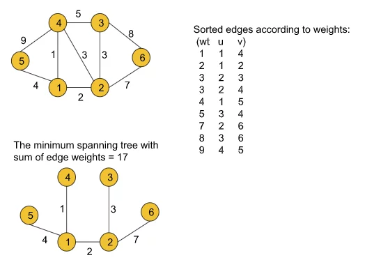
1. Kruskal's Algorithm

Approach:
We will be implementing Kruskal’s algorithm using the Disjoint Set data structure that we have previously learned.
Now, we know Disjoint Set provides two methods named findUPar()(This function helps to find the ultimate parent of a particular node) and Union(This basically helps to add the edges between two nodes).

The algorithm steps are as follows:

• First, we need to extract the edge information(if not given already) from the given adjacency list in the format of (wt, u, v) where u is the current node, v is the adjacent node and wt is the weight of the edge between node u and v and we will store the tuples in an array.
• Then the array must be sorted in the ascending order of the weights so that while iterating we can get the edges with the minimum weights first.
• After that, we will iterate over the edge information, and for each tuple, we will apply the following operation:
  • First, we will take the two nodes u and v from the tuple and check if the ultimate parents of both nodes are the same or not using the findUPar() function provided by the Disjoint Set data structure.
  • If the ultimate parents are the same, we need not do anything to that edge as there already exists a path between the nodes and we will continue to the next tuple.
  • If the ultimate parents are different, we will add the weight of the edge to our final answer(i.e. mstWt variable used in the following code) and apply the union operation(i.e. either unionBySize(u, v) or unionByRank(u, v)) with the nodes u and v. The union operation is also provided by the Disjoint Set.
• Finally, we will get our answer (in the mstWt variable as used in the following code) successfully.

def find(parent, x):
	if x == parent[x]:
		return x
	temp = find(parent, parent[x])
	parent[x] = temp
	return temp

def unionByRank(parent, rank, x, y):
	px = find(parent, x)
	py = find(parent, y)
	if px == py: return
	if rank[px] > rank[py]:
		parent[py] = px
	elif rank[px] < rank[py]:
		parent[px] = py
	else:
		parent[px] = py
		rank[py] += 1
	
#  Applying Kruskal algorithm
def kruskal_algo(self):
	result = []
	i, e = 0, 0 #edge_iterator, mst_edge_cnt
	self.graph = sorted(self.graph, key=lambda item: item[2])
	parent = []
	rank = []
	for node in range(self.V):
		parent.append(node)
		rank.append(0)
	while e < self.V - 1:
		u, v, w = self.graph[i]
		i = i + 1
		x = self.find(parent, u)
		y = self.find(parent, v)
		if x != y:
			e = e + 1
			result.append([u, v, w])
			self.apply_union(parent, rank, x, y)
	for u, v, weight in result:
		print("%d - %d: %d" % (u, v, weight))

Time Complexity: O(N+E) + O(E logE) + O(E4α2) where N = no. of nodes and E = no. of edges. O(N+E) for extracting edge information from the adjacency list. O(E logE) for sorting the array consists of the edge tuples. Finally, we are using the disjoint set operations inside a loop. The loop will continue to E times. Inside that loop, there are two disjoint set operations like findUPar() and UnionBySize() each taking 4 and so it will result in 42. That is why the last term O(E4*2) is added.

Space Complexity: O(N) + O(N) + O(E) where E = no. of edges and N = no. of nodes. O(E) space is taken by the array that we are using to store the edge information. And in the disjoint set data structure, we are using two N-sized arrays i.e. a parent and a size array (as we are using unionBySize() function otherwise, a rank array of the same size if unionByRank() is used) which result in the first two terms O(N).

Many more things are yet to be added like

• Strongly COnnected components by Kosarajus algo
• Tarjans(bridges)
• Articulation points

ARTICULATION POINTS

def ArticulationPoints(graph, v, e):
    
    visited = [False]*(v+1)
    parent = [-1]*(v+1)
    disc = [sys.maxsize]*(v+1)
    low = [sys.maxsize]*(v+1)
    artPoint = [False]*(v+1)
    
    discoveryTime = [0]
    actualSrc = [1]
    childrensOfActualSrc = [0]
    
    def AP_DFS(graph,v,e,src):
        visited[src] = True
        disc[src] = discoveryTime[0]
        low[src] = discoveryTime[0]
        discoveryTime[0] += 1
        
        neighbours = graph[src]
        
        for nbr in neighbours:
            if nbr == parent[src]:
                continue
            if visited[nbr] == True:
                low[src] = min(low[src], disc[nbr])
            else:
                parent[nbr] = src
                
                if src == actualSrc[0]:
                    childrensOfActualSrc[0] += 1
                    
                AP_DFS(graph, v, e, nbr)
                
                low[src] = min(low[src], low[nbr])
                
                if src != actualSrc[0]:
                    if disc[src] <= low[nbr]:
                        artPoint[src] = True
    AP_DFS(graph, v, e, 1)
    
    totalArticulationPoints = 0
    for i,node in enumerate(artPoint):
        if i != 1:
            if node == True:
                totalArticulationPoints+=1
                
    if childrensOfActualSrc[0] > 1:
        totalArticulationPoints+=1
    
    return totalArticulationPoints
    
import sys
t = int(input())
for _ in range(t):
    v, e = map(int,input().split())
    
    graph = {}
    for i in range(1,v+1):
        graph[i] = []
        
    for ed in range(e):
        s, d = map(int,input().split())
        graph[s].append(d)
        graph[d].append(s)

Critical connections- Bridges

class Solution:
    def criticalConnections(self, n: int, connections: List[List[int]]) -> List[List[int]]:
        v = n
        graph = {}
        for i in range(0,n):
            graph[i] = []

        for ed in connections:
            s, d = ed[0], ed[1]
            graph[s].append(d)
            graph[d].append(s)
    
        visited = [False]*(v)
        parent = [-1]*(v)
        disc = [sys.maxsize]*(v)
        low = [sys.maxsize]*(v)
        artPoint = [False]*(v)

        discoveryTime = [0]
        actualSrc = [0]
        childrensOfActualSrc = [0]
        
        result = []

        def AP_DFS(graph,v,src):
            visited[src] = True
            disc[src] = discoveryTime[0]
            low[src] = discoveryTime[0]
            discoveryTime[0] += 1

            neighbours = graph[src]

            for nbr in neighbours:
                if nbr == parent[src]:
                    continue
                if visited[nbr] == True:
                    low[src] = min(low[src], disc[nbr])
                else:
                    parent[nbr] = src

                    if src == actualSrc[0]:
                        childrensOfActualSrc[0] += 1

                    AP_DFS(graph, v, nbr)

                    low[src] = min(low[src], low[nbr])

                    if disc[src] < low[nbr]:
                        artPoint[src] = True
                        result.append([src,nbr])
                            
        AP_DFS(graph, v, 0)
        # print(artPoint)

        totalArticulationPoints = 0
        for i,node in enumerate(artPoint):
            if i != actualSrc[0]:
                if node == True:
                    totalArticulationPoints+=1

        if childrensOfActualSrc[0] > 1:
            totalArticulationPoints+=1

        return result
	

Please UPVOTE if you like it. ALso add your feedbacks and all in comments.